Language Modelling

Authors of (Liu et al., 2018) suspect that, for monolingual text-to-text tasks, redundant language information is re-learned by both the encoder and decoder. In the paper, they perform supervised learning for the task of summarizing Wikipedia documents. The input is the top extracted document for a given topic, concatenated with a special token and the expected summary. They propose that the task can be performed in two stages: (1) extraction of top Wikipedia documents related to a topic using methods such as Identity, TF-IDF, TextRank, SumBasic, and a "cheating" baseline; and (2) abstraction through language modeling using a decoder-only Transformer model.

They prove the claim by performing a sequence transduction problem from very long input sequences (up to \(L = 11000\)) to medium output sequences (typically less than 500).

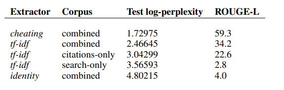
The figure compares different extractive methods on the combined corpus using an input length of \(L = 500\) (medium-sized token length). Among the evaluated methods, the "cheating" strategy performs the best.

Decoder-only Transformer

Let the sequence be represented as \( (w_1, \ldots, w_{n+\eta+1}) = (m_1, \ldots, m_n, \delta, y_1, \ldots, y_\eta) \), where \( \delta \) is a special separator token. The model is trained to predict the next token given the previous ones:

\( p(w_1, \ldots, w_{n+\eta}) = \prod_{j=1}^{n+\eta} p(w_j \mid w_1, \ldots, w_{j-1}) \)

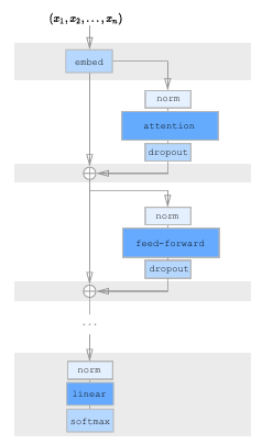
The D-TF model eliminates the encoder from the original Transformer architecture, thereby reducing both parameter count and time complexity by half. The input and output sequences are merged into a single sequence using a special separator token. To predict the next token, both the input m and output y are given as input, with future tokens masked out to enable causal training.

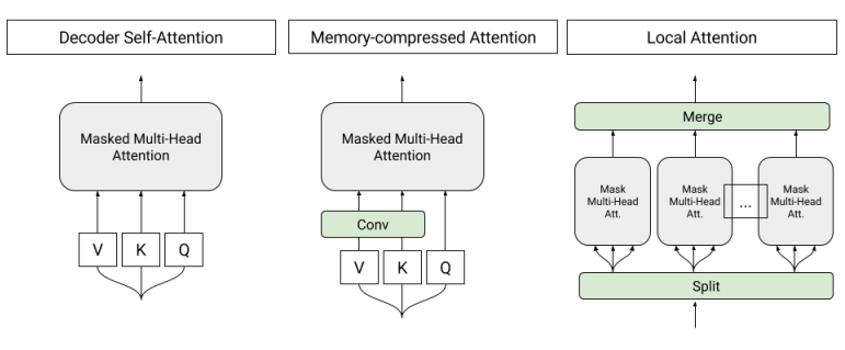
Transformer Decoder with Memory-Compressed Attention (T-DMCA)

Local Attention Block: This block involves splitting the input sequence into segments of 256 tokens, which are then fed into multi-head attention in parallel and separately.

Memory-Compressed Attention Block: After projecting the input tokens into query, key, and value spaces, strided convolution is applied before passing the result to multi-head attention. This reduces parameters via a compression factor. Strided convolution uses kernels of size 3 with a stride of 3. Unlike local attention, memory-compressed attention captures global information across the entire sequence, similar to the original Transformer.

The final architecture is a 5-layer network (L-M-L-M-L), alternating between local attention (L) layers and memory-compressed attention (M) layers (compared to 6 identical layers in Vaswani et al., (2017)). In some experiments, a Mixture of Experts (MoE) layer is added to increase the model’s capacity.

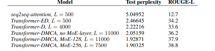
The performance of the best models from each architecture, evaluated using the combined corpus and tf-idf extractor, is shown above. As noted in Table 4, the seq2seq-attention baseline performs significantly worse than Transformer-based models on this task. As seen in Figure, the Transformer encoder-decoder (T-ED) architecture steadily improves performance up to an input length \(L = 500{-}1000\), but fails to learn at \(L = 2000\).

This limitation motivated the use of the Transformer-Decoder (D-TF), which successfully trained up to \(L = 4000\) before hitting memory limits on machines with 16GB GPU RAM (NVIDIA P100). By applying the T-DMCA modifications, the model was able to scale up to \(L = 11,000\), with continued improvements in performance.

Additionally, incorporating a Mixture of Experts (MoE) layer enhanced model capacity at high input lengths. For instance, at \(L = 11,000\), adding 128 experts reduced log-perplexity from 2.05 to 1.93. The best-performing model used 256 experts at \(L = 7500\) and achieved a log-perplexity of 1.90. (Note: 256 experts at \(L = 11,000\) could not be run due to memory constraints.)

Generative Pre-Training (GPT)

One estimate suggests that text data — including web pages, social media posts, emails, and more — could total 100–200 terabytes, according to Educating Silicon. However, this is just a fraction of the data generated daily (measured in zettabytes, ZB). Unsupervised, unannotated corpora can be used to learn rich representations, which are then fine-tuned on smaller labeled datasets for specific tasks. Word embeddings trained on large unlabeled corpora already demonstrate this principle; future work aims to extend these embeddings to capture higher-level semantics and richer context.

GPT proposes a semi-supervised technique that combines unsupervised pre-training of a neural network using a language modeling objective with supervised fine-tuning on task-specific labeled data.

Unsupervised Pre-Training

For pre-training, the authors use a decoder-only Transformer, trained to predict each token in sequence using the same autoregressive objective described earlier.

Supervised Fine-Tuning

Given a labeled dataset C of input–label pairs (x₁, x₂, …, xₘ; y), the fine-tuning objective is:

Lfine-tuning(C) = ∑(x,y)∈C log P(y | x₁, x₂, …, xₘ)

In practice, they also retain the auxiliary language modeling objective to improve generalization and convergence speed:

L = Lfine-tuning(C) + λ · Lpre-training(C)

Only the final linear layer’s weights (Wy) are initialized anew for each task; all other parameters come from pre-training.

Application to Language Understanding Tasks

GPT is evaluated on four types of tasks: natural language inference, question answering, semantic similarity, and text classification. Rather than redesigning the architecture for each task, they simply concatenate task-specific inputs and delimiters to the pre-trained model’s input sequence.

• Classification: The input sequence is passed directly through the model, and the final hidden state of a special classification token is fed to a linear layer.
• Textual Entailment: Concatenate the premise p and hypothesis h with a delimiter token (e.g., [SEP]) in between.
• Semantic Similarity: Process both sentence orderings independently (with a delimiter), producing two vectors h₁ and h₂; sum them element-wise before the final linear layer.
• Question Answering: For each candidate answer a_k, concatenate [context] ; [question] ; [SEP] ; ak, run each through the model, and normalize scores with softmax.

Key Takeaways

1. Transferring more Transformer layers during fine-tuning incrementally improves performance, suggesting that deeper contextual representations are beneficial. 2. Ablation studies show that retaining the auxiliary language modeling objective during fine-tuning stabilizes training and helps performance, especially on larger downstream datasets. Smaller datasets benefit less from the auxiliary objective.

GPT-2

GPT-2 is an extension of the original GPT, which was a smaller model. GPT-2 is a 1.5B parameter model designed to enhance the zero-shot capabilities of large language models that can later be fine-tuned for specific tasks. The core idea is to treat language modeling as a conditional probability estimation problem, p(output | input), for a given task. To generalize this to a multi-task setting, the model should be conditioned not just on the input but also on the task description. Unlike previous approaches that made architectural changes for different tasks, GPT-2 uses a single unified architecture and relies on scaling and training on diverse data.

Training Details: To train GPT-2, the authors used a massive corpus of web text from various domains and contexts. While datasets like Common Crawl are often used, they suffer from quality issues. To address this, the authors created a new dataset called WebText, which emphasizes quality over quantity. They scraped all outbound links from Reddit posts that received at least 3 karma points, treating karma as a proxy for human approval or relevance. The WebText dataset does not include Wikipedia, and after preprocessing and filtering, it contains 8 million documents totaling 40 GB of text.

Four models were pre-trained on WebText with varying parameter sizes. The largest, with 1.5 billion parameters, is known as GPT-2. These models were then fine-tuned on downstream tasks such as reading comprehension, summarization, and question answering. GPT-2 achieved state-of-the-art performance in several tasks and performed comparably well on machine translation without task-specific architectural changes.

Language Generation

Problem with Transformer: Consider tasks like language modeling on text, image, or audio data. The goal is to use previous inputs to generate a categorical distribution over a vocabulary of size v using the softmax function, i.e., to predict the next token in the sequence. The joint probability of a sequence x = x₁, x₂, ..., xₙ is modeled as:

p(x) = ∏i=1n p(xᵢ | x₁, ..., xᵢ₋₁; θ)

During training, we optimize the parameters θ to maximize the likelihood of the data. However, the problem arises when using standard Transformers (encoder-decoder or decoder-only) because the self-attention block has a computational complexity of O(n²), where n is the sequence length.

To improve performance, large language models require a larger context window — meaning longer sequences — which makes this O(n²) cost prohibitive. Therefore, modifications to the original Transformer architecture are needed to make it scalable and efficient on massive datasets.

Factorized Self-Attention

The authors experimented with a 128-layer full-attention Transformer trained on CIFAR-10. They observed the following:

• Early layers learned local patterns (like neighboring pixels — similar to CNNs).
• Mid layers developed patterns like row and column attention — factorizing attention along 2D structure.
• Later layers showed sparse or even global attention patterns, often in data-dependent ways.

These findings motivated the idea of introducing deliberate sparsity in attention while maintaining performance, this is similar to CNNs which build global understanding from local connectivity.

In a dense Transformer, each token (e.g., image patch or word) is projected into queries, keys, and values using weight matrices. Each output is a weighted sum of the values, with weights based on the similarity between the query and keys. In full self-attention, every token xᵢ attends to all previous tokens {x₁, x₂, ..., xᵢ} (autoregressive masking):

x₁ → x₂ → x₃ → ... → xₙ

This requires O(n²) computations. For n = 16,384, that leads to over 256 million attention computations.

Sparse Transformer: Instead of full attention, the Sparse Transformer uses p separate attention heads. Each head attends only to a subset of tokens — similar to how CNN filters cover a local region. Over multiple layers, these sparse heads can still pass information globally. For any output token i and any input token j, there exists a path of attention through intermediate tokens of at most p+1 steps to connect j to i.

Computational Complexity

In sparse attention:

• Each token attends to only n/p tokens instead of n.
• So, per-token computation is O(n/p).
• Across n tokens: O(n × n/p) = O(n² / p).

This is cheaper than full attention as long as p > 1. If we choose p = √n (a common choice), then:

O(n² / √n) = O(n · √n)

This significantly reduces compute cost for long sequences (e.g., n = 16,384).

Two-dimensional Factorized Attention

Strided Attention

For structured data like images or music — where nearby pixels or notes are most relevant — we can use strided attention to focus on local patterns. This involves two attention heads:

• A(1)i = {i−l, ..., i−1} → attends to recent l tokens (local context)
• A(2)i = {j | j mod l = 0} → attends to every lth token (strided/global context)

This approach aligns well with structured data formats and allows efficient sparse attention.

Fixed Attention

For unstructured data like text — where context can shift rapidly and skipping words can cause errors — strided attention may fail to capture dependencies. Instead, fixed attention allows specific summary blocks to be attended by future tokens.

For example, if stride l = 128 and block size c = 8:

• Positions after 128 attend to tokens 120–128
• Positions after 256 attend to tokens 248–256
• And so on...

This allows each block of c tokens to act as a summary for a window, and subsequent tokens can attend to these summaries for long-term dependencies. Note: This increases compute by a factor of c compared to strided attention — a tradeoff for more reliable information flow in non-periodic data like language.

Sparse Transformer

Let’s see how factorized attention is used in Sparse Transformers. Below are the key architectural changes compared to the original Transformer:

1. Factorized Attention Heads: The transformer has many residual blocks: Block 0, Block 1, Block 2, etc. Use every attention types alternately in every block. So, if you have p = 2 attention types (e.g., strided and fixed), then:

• Block 0 → use attention type A(0 mod 2) = A(0) → strided
• Block 1 → use attention type A(1 mod 2) = A(1) → fixed
• Block 2 → back to strided, and so on...

Mathematically, it can be represented as:

attention(X) = Wp · attend(X, A(r mod p))

• r = current residual block number
• p = number of attention types (e.g., 2)
• A(i) = attention pattern (like strided or fixed)

Pros: Very efficient; each block is simple.
Cons: One block only sees one pattern at a time.

Merged Attention Head: Instead of rotating attention heads, we combine all attention patterns into one merged head. Each token attends to the union of all sparse sets.

attention(X) = Wp · attend(X, ⋃ A(m)), for m = 1 to p

Look at everything that all the sparse heads would have attended to using one combined attention operation.

Pros: Gets richer information per block.
Cons: Slightly more computation since each head attends to more positions.

Multi-Head Attention (Standard Transformer Style): This is inspired by traditional method from Vaswani et al. (2017). In multi-head attention, the model uses nh parallel attention heads, where each head attends to a different subset of the input using its own sparse pattern, denoted as A(i). These attention operations are computed in parallel, and their outputs are then concatenated along the feature dimension to form the final output of the attention layer.

attention(X) = Wp · concat(attend(X, A(i))) for i = 1 to nh

Pros: Allows parallelism and flexibility.
Cons: May use more GPU memory when computed in parallel.

2. Scaling to Hundreds of Layers: Training very deep transformers can be difficult due to vanishing or exploding gradients. To handle this, the Sparse Transformer uses ResNet-style pre-activation residual blocks around both the attention and feed-forward layers.

To keep activations stable as the number of layers increases, they scale certain weight matrices by

1 / √(2N)

where N is the number of layers. This helps ensure that outputs neither vanish nor explode as they propagate through the network.

3. Modeling Diverse Data Types: Transformers are location-agnostic by default, so positional embeddings are essential—especially for sparse attention patterns. The model adds nemb = ddata or nemb = dattn learned embeddings to each input, depending on whether it's data- or attention-structure based:

embed(XWe) = xiWe + Σj=1 to nemb oi(j) · Wj

• For images: ddata = 3 → row, column, and channel of each byte.
• For text/audio: dattn = 2 → row and column index (assuming 2D layout with stride).

4. Saving Memory by Recomputing Attention Weights: Self-attention layers consume a lot of memory, especially for long sequences. To reduce memory usage, Sparse Transformers use gradient checkpointing.

During the forward pass, the model saves only a few intermediate activations, known as checkpoints, while discarding the rest to reduce memory usage. Then, during the backward pass, the model recomputes the discarded layers on-the-fly as needed to calculate gradients.

For Example:

Forward Pass:
  Layer 1 → Save
  Layer 2 → Discard
  Layer 3 → Save
  Layer 4 → Discard
  Layer 5 → Discard
  Layer 6 → Save final output

Backward Pass:
  To backprop through Layers 2–3 → Recompute using Layer 1 checkpoint
  To backprop through Layers 4–5 → Recompute using Layer 3 checkpoint

Since dropout involves randomness, recomputing outputs could yield different results unless random seeds are controlled. To avoid this complexity, the authors apply dropout only at the end of residual blocks—not inside attention layers.

5. Mixed-Precision Training: Sparse Transformer uses mixed-precision training to accelerate training and reduce memory usage.

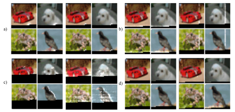
Results

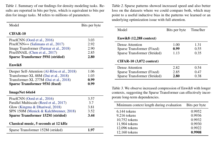
The Sparse Transformer achieved state-of-the-art results across all modalities. A few key observations include that, for language generation, performance improves significantly when the context window is large, as shown in Table 3. As discussed in the previous section, the choice of sparse attention pattern depends on the nature of the dataset. Strided attention performs well on structured datasets such as images or music, while it is less effective for unstructured data like text, where fixed attention is more suitable.

References

1. Radford et al (2019). Language models are unsupervised multitask learners. OpenAI.
2. Radford et al (2018). Improving Language Understanding by Generative Pre-Training. OpenAI.
3. Child et al. (2019). Generating long sequences with sparse transformers. In Advances in Neural Information Processing Systems (NeurIPS).
4. Vaswani et al. (2017), Attention Is All You Need. In Advances in Neural Information Processing Systems (NeurIPS).
5. Liu et al. (2018), Generating Wikipedia by Summarizing Long Sequences, International Conference on Learning Representations (ICLR).