Generative Adversarial Networks (GANs) started with vanilla GANs—uncontrolled models that generate data by competing generator and discriminator networks, but without specific output control. To enable targeted generation, conditional GANs (cGANs) were developed, which use extra information like class labels to guide both the generator and discriminator. This allows cGANs to produce data with desired attributes, supporting advanced applications such as image-to-image translation and controlled synthesis
1. Vanilla Generative Adversarial Network
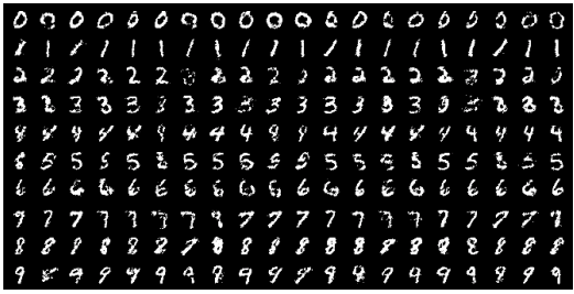
GANs (Generative Adversarial Networks) are implicit generative models: rather than explicitly computing or modeling likelihood functions, they aim to learn how to sample from the underlying data distribution. The objective is for the generator to produce samples that closely resemble the true data distribution, without ever directly estimating the probability density or likelihood.
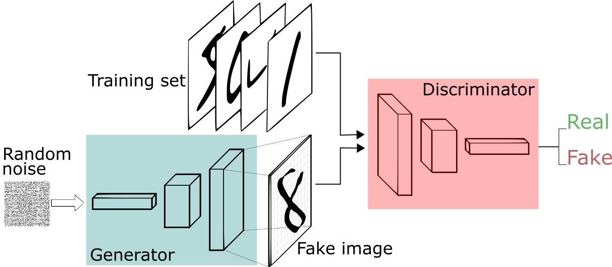
A normally distributed random variable \( z \sim \mathcal{N}(0, I) \) is passed through the generator network to produce fake images with a similar distribution to the real dataset. To train the generator, GANs use a zero-sum loss function, encouraging the generator to produce images that the discriminator classifies as real.
Train the generator \( G \) such that the discriminator \( D \) misclassifies the generated sample \( \hat{x} \) into class 1 (real data and 0 for fake gernated sample), making it indistinguishable from real data \( x \sim p_{\text{data}} \).
Discriminator Objective \( O_1 \)
Train discriminator \( D \) to maximize the log probability of correctly classifying real samples:
Generator Objective \( O_2 \)
Train generator \( G \) to minimize the probability that the discriminator correctly classifies generated samples as fake:
Training Strategy
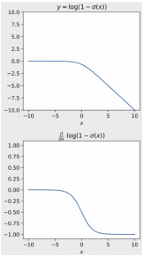
If a pretrained discriminator is used initially, it might confidently classify all generated images as fake, resulting in \( \log(1 - D(G(z))) = \log(1 - 0) = 0 \), which leads to zero gradient for training the generator.
Therefore, it is essential to train both the generator and the discriminator alternately using different mini-batches. This avoids collapse and ensures both models improve progressively.
The minimax objective of a Generative Adversarial Network is:
Expanding the expectations using the change of variables:
Now take the max inside the integral:
Let \( y = D(x), \quad a = p_{\text{data}}(x), \quad b = p_G(x) \). Define:
To maximize \( f(y) \), take the derivative and set it to zero:
Optimal Discriminator \( D^*_G(x) \)
Substituting back:
Now substitute this optimal discriminator into the original objective:
Rewriting the expression using expectations:
Multiply numerator and denominator by 2:
Which leads to the final expression involving KL divergence:
Jensen–Shannon Divergence (JSD)
So the GAN objective simplifies to:
This expression is minimized when
since Jensen–Shannon divergence is non-negative and equals 0 only when the two distributions are identical.
2. Deep Convolution Generative Adversarial Network (DCGAN)
DCGAN bridge the gap between the unsupervised method and success of Convolutional Neural Networks stablize the training of Vanilla GANs.Architectural Guidelines for Stable GAN Training:
-
Replaces deterministic spatial pooling functions (e.g., max pooling) with strided convolutions
- Allows the network to learn spatial downsampling
-
Removes fully connected hidden layers
- Supports deeper and more scalable architectures
-
Batch Normalization in both Generator and Discriminator
- Prevents generator collapse
- Enables stable gradient flow in deeper networks
- Not applied at the output layer of the generator or input layer of the discriminator
-
Non-linear Activations:
- Generator: ReLU activations in all layers except the output
- Discriminator: Leaky ReLU activations with slope 0.2
-
Output Activations:
- Generator: tanh
- Discriminator: sigmoid
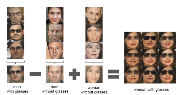
DCGAN demonstrates an interesting experiment with the latent space: when the latent vector of a man with glasses is subtracted from that of a man, and the result is added to the latent vector of a woman, the resulting vector generates images of women with glasses.
3. Conditional Generative Adversarial Network (cGAN)
So far, we have seen the impressive generation capabilities of GANs. However, a key limitation is the lack of control over what the GAN generates, for example, generating images of a specific class or outputs from other modalities like text.
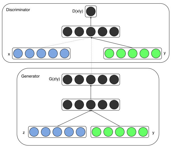
(cGANs) address this limitation by introducing an additional conditioning variable y, which can be a class label, text embedding, or any other feature vector derived from a different modality. In this framework, both the generator and the discriminator are conditioned on y:
- Generator: The latent noise vector
zis concatenated withy, enabling the model to learn the conditional probability distribution \( p(x|y) \). - Discriminator: Both the generated/real sample
xand the conditioning variableyare provided as input, allowing the model to evaluate whetherxis a realistic sample giveny.
The objective function for a conditional GAN becomes:
\[ \min_G \max_D V(D, G) = \mathbb{E}_{x \sim p_{\text{data}}(x)}[\log D(x|y)] + \mathbb{E}_{z \sim p_z(z)}[\log(1 - D(G(z|y)))] \]
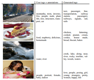
cGANs have been successfully used to generate both unimodal outputs (e.g., generating images from class labels) and multimodal outputs (e.g., generating descriptive tags from images). Here, the author tried to demonstrate automated tagging of images, with multi-label predictions, using conditional adversarial nets to generate a (possibly multi-modal) distribution of tag-vectors conditional on image features. They used the skip-model trained on the dictionary of size 247465 and the convolution networks to generate tags and images generation respectively.
4. Cycle Generative Adversarial Network (CycleGAN)
CycleGAN enables image-to-image translation between two visual domains without requiring paired training examples. When trained on two unpaired image collections, CycleGAN learns to capture the domain-specific characteristics of each and translates between them. The model assumes that there is some underlying shared structure between domains — for example, both being different renderings or styles of the same scene — and seeks to learn a mapping between them.
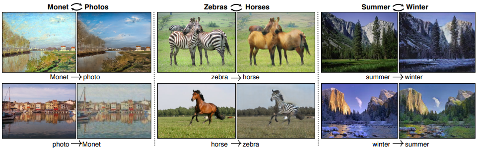
CycleGAN has become widely popular for tasks like style transfer, object transfiguration, season conversion, and photo enhancement. Its unique capability to perform translations without paired data makes it powerful for real-world applications where aligned datasets are unavailable.
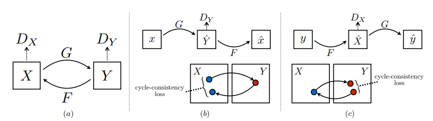
A key insight from CycleGAN is that adversarial loss alone is insufficient to ensure meaningful translations. The model might map multiple inputs to the same output or introduce artifacts. To solve this, CycleGAN introduces the concept of cycle consistency, which enforces that translating from one domain to another and back again should yield the original image ideally. This is analogous to translating a sentence from English to French and then back to English — the result should closely resemble the original sentence.
Adversarial Loss
The adversarial loss ensures that the generated images from one domain are indistinguishable from real images in the target domain.
\[ \mathcal{L}_{GAN}(G, D_Y, X, Y) = \mathbb{E}_{y \sim p_{data}(y)}[\log D_Y(y)] + \mathbb{E}_{x \sim p_{data}(x)}[\log(1 - D_Y(G(x)))] \]
Similarly, for the reverse direction:
\[ \mathcal{L}_{GAN}(F, D_X, Y, X) = \mathbb{E}_{x \sim p_{data}(x)}[\log D_X(x)] + \mathbb{E}_{y \sim p_{data}(y)}[\log(1 - D_X(F(y)))] \]
Cycle Consistency Loss
To preserve the content between translations, CycleGAN uses a cycle consistency loss. This ensures that: \[ F(G(x)) \approx x \quad \text{and} \quad G(F(y)) \approx y \]
The cycle consistency loss is defined as:
\[ \mathcal{L}_{cyc}(G, F) = \mathbb{E}_{x \sim p_{data}(x)}[\|F(G(x)) - x\|_1] + \mathbb{E}_{y \sim p_{data}(y)}[\|G(F(y)) - y\|_1] \]
Notice that our model can be viewed as training two “autoencoders” [20]: we learn one autoencoder F o G : X -> X jointly with another G o F : Y -> Y. However, these autoencoders each have special internal structures: they map an image to itself via an intermediate representation that is a translation of the image into another domain. Such a setup can also be seen as a special case of “adversarial autoencoders”, which use an adversarial loss to train the bottleneck layer of an autoencoder to match an arbitrary tarm get distribution. In our case, the target distribution for the X-> Xautoencoderisthat of the domain Y.
Full Objective
The full objective combines both adversarial and cycle consistency losses:
\[ \mathcal{L}(G, F, D_X, D_Y) = \mathcal{L}_{GAN}(G, D_Y, X, Y) + \mathcal{L}_{GAN}(F, D_X, Y, X) + \lambda \cdot \mathcal{L}_{cyc}(G, F) \]
The optimization problem becomes:
\[ G^*, F^* = \arg\min_{G, F} \max_{D_X, D_Y} \mathcal{L}(G, F, D_X, D_Y) \]
Stabilizing Training with Least Squares Loss
To improve training stability and gradient flow, CycleGAN replaces the binary cross-entropy loss with a least squares loss. This change modifies the generator and discriminator objectives as follows:
- Generator loss: \( \mathbb{E}_{x \sim p_{data}(x)}[(D(G(x)) - 1)^2] \)
- Discriminator loss: \( \mathbb{E}_{y \sim p_{data}(y)}[(D(y) - 1)^2] + \mathbb{E}_{x \sim p_{data}(x)}[(D(G(x)))^2] \)
This formulation leads to smoother gradients, helping the model learn more effectively, and avoids issues like vanishing gradients often seen in vanilla GAN training.
In summary, CycleGAN elegantly solves the unpaired image-to-image translation problem by combining adversarial training with cycle consistency, enabling powerful and flexible cross-domain generation without requiring paired data.
References
- NPTEL Course, "Deep Learning for Computer Vision [Online].* Available: https://www.youtube.com/playlist?list=PLyqSpQzTE6M_PI-rIz4O1jEgffhJU9GgG"
- Radford, A., et al. (2016). Unsupervised representation learning with deep convolutional generative adversarial networks. arXiv preprint arXiv:1511.06434.
- Mirza, M., et al. (2014). Conditional generative adversarial nets. arXiv preprint arXiv:1411.1784.
- Zhu, J. Y., et al. (2017). Unpaired image-to-image translation using cycle-consistent adversarial networks. In Proceedings of the IEEE International Conference on Computer Vision (ICCV) (pp. 2223–2232).
- Xie, Pengtao. (2025). ECE 285 Deep Generative Models. Electrical and Computer Engineering, UCSD.