NLP Preprocessing Concepts
1. Tokenization
Tokenization is the process of breaking down text into smaller units called tokens.
Types of Tokenization:
- Character Tokenization:
“Project A is done.” ⇒ ‘P’, ‘r’, ‘o’, ‘j’, ‘e’, ‘c’, ‘t’, ‘ ’, ‘A’, ... - Word Tokenization:
“Project A is done.” ⇒ ‘Project’, ‘A’, ‘is’, ‘done’, ‘.’ - Sentence Tokenization:
“Project A is done. We will start Project B tomorrow.”
⇒ ‘Project A is done.’, ‘We will start Project B tomorrow.’
Common libraries: re, nltk, spacy
2. Stemming
Stemming reduces words to their base or root form (sometimes not a real word):
- meeting, meets, met ⇒ meet
- connected, connecting ⇒ connect
- history, historical ⇒ histori (incorrect root)
3. Lemmatization
Lemmatization also reduces words to their base form but ensures the result is a valid word:
- connected, connecting ⇒ connect
- was, were ⇒ be
- history, historical ⇒ history (preserves meaning)
4. Stopwords
Stopwords are common words that do not add significant meaning to text (e.g., “the”, “is”, “an”, “we”).
Example sentence before and after removing stopwords:
- Original: “We have completed the project successfully.”
- After stopword removal: “completed project successfully”
5. Case Sensitivity
Text like “Email” and “email” are the same for humans but not for machines.
Lowercasing: “Project EMAIL” ⇒ “project email”
6. Bag-of-Words (BoW)
BoW represents documents as a collection of word frequencies without considering order or grammar.
Example Emails (Documents):
- Doc1: “The project report was submitted.”
- Doc2: “She submitted the final report.”
- Doc3: “We reviewed the project and the report.”
Binary BoW:
| project | report | submitted | |
|---|---|---|---|
| Doc1 | 1 | 1 | 1 |
| Doc2 | 0 | 1 | 1 |
| Doc3 | 1 | 1 | 0 |
Numerical BoW (word counts):
| project | report | submitted | |
|---|---|---|---|
| Doc1 | 1 | 1 | 1 |
| Doc2 | 0 | 1 | 1 |
| Doc3 | 1 | 2 | 0 |
Note: BoW does not capture word meaning or order.
7. Term Frequency-Inverse Document Frequency (TF-IDF)
TF (Term Frequency):
| project | report | submitted | |
|---|---|---|---|
| Doc1 | 1/3 | 1/3 | 1/3 |
| Doc2 | 0 | 1/2 | 1/2 |
| Doc3 | 1/3 | 2/3 | 0 |
IDF (Inverse Document Frequency):
| Term | IDF |
|---|---|
| project | log(3/2) |
| report | log(3/3) = 0 |
| submitted | log(3/2) |
TF-IDF Scores:
| project | report | submitted | |
|---|---|---|---|
| Doc1 | 1/3 × log(3/2) | 0 | 1/3 × log(3/2) |
| Doc2 | 0 | 0 | 1/2 × log(3/2) |
| Doc3 | 1/3 × log(3/2) | 0 | 0 |
TF-IDF helps identify important words across documents by balancing term frequency with how rare a term is in the corpus. It still does not capture word order or deep semantics.
So far, all the techniques treat a token as separate atomic unit of which sentences are made and mostly of them do not capture the semantic relationship that is usually present in the corpus or vocabulury. What if we could have a continuous embedding space for words wherein vector(King) - vector(Man) + vector(Woman) would result into a vector that is similar to vector(Queen) in the embedding space. This can then be used for some downstream tasks using the neural networks that capture long range dependencies for machine translation, etc.
8. Word2Vec - Word Embedding
Word2Vec, proposed by Mikolov et al., introduces two techniques for learning these representations: Continuous Bag of Words (CBOW) and Skip-Gram. Both architectures use three layers: an input layer, a projection layer, and an output layer. They showed that it is possible to train the models even on corpora with one trillion words (virtually all available data as of 2013), for basically unlimited size of the vocabulary.
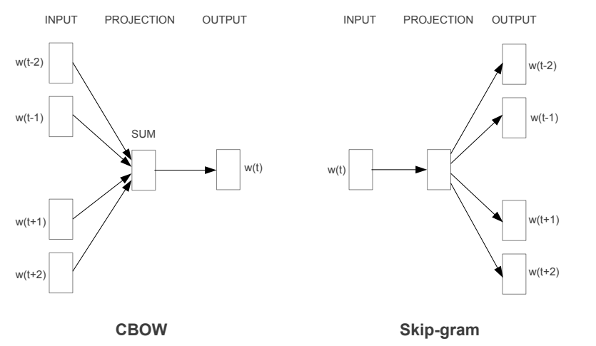
Continuous Bag of Words (CBOW)
In CBOW, for a window size of 2, the surrounding context words w(t-2), w(t-1), w(t+1), and w(t+2) are used to predict the target word w(t). The input vectors are one-hot encoded representations of the vocabulary. The network aggregates these to produce a prediction via a softmax layer.
Skip-Gram
Skip-Gram works in the reverse manner. Given a center word w(t), the model attempts to predict the surrounding context words in the window. This method performs well on semantic relationships and is particularly effective for rare words when trained on large corpora.
In both these methods the hidden task is to learn the weights of the projection layer that learn the vector embedding space.
CBOW vs. Skip-Gram
The choice of the CBOW or Skip Gram method depends on the use case. The pros and cons are as listed below:
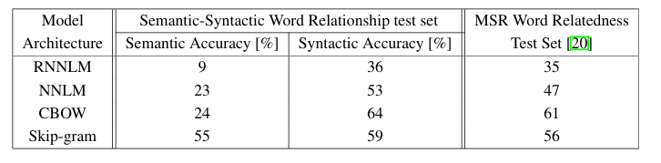
- Skip-Gram generally achieves higher accuracy, especially on semantic relationships and with rare words, when trained on large corpora and high-dimensional embeddings.
- CBOW is computationally more efficient and performs well for frequent words and syntactic tasks, though it may underperform Skip-Gram on semantics.
Semantic vs. Syntactic Accuracy
In the original Word2Vec paper, Mikolov et al. defined two evaluation metrics:
- Semantic accuracy: Measures the model’s ability to capture meaning-based relationships (e.g., “Paris” is to “France” as “Berlin” is to “Germany”).
- Syntactic accuracy: Measures how well the vectors capture grammatical or morphological relationships (e.g., “walking” is to “walked” as “swimming” is to “swam”).
The authors evaluated their model on a benchmark dataset of 8,869 semantic and 10,675 syntactic analogy questions. A correct prediction means the nearest word vector exactly matches the expected answer; synonyms are not accepted.
- Fails to capture the global context across long sentences or paragraphs, as it considers only a limited window of surrounding words at a time.
- While it performs well on morphological/ syntactic relationships, it may not effectively model deeper semantic meaning or long-range dependencies.
Global Co-occurrence Statistics in GloVe
As discussed earlier, the Word2Vec model primarily leverages local context windows during training and does not fully utilize the global co-occurrence statistics available in the corpus. Global Vectors for Word Representation (GloVe) addresses this limitation by explicitly incorporating global co-occurrence information to learn more informative word embeddings.
To evaluate the quality of these embeddings, GloVe uses an analogy task consisting of 19,544 questions, divided into two categories: semantic and syntactic analogies.
- Semantic analogies capture relationships between named entities, such as: "Athens is to Greece as Berlin is to ?"
- Syntactic analogies reflect grammatical or morphological patterns, such as: "Dance is to dancing as fly is to ?"
To solve an analogy of the form “a is to b as c is to ?”, the model computes a target word vector using the following expression:
\( \vec{d} = \vec{b} - \vec{a} + \vec{c} \)
The model then selects the word d whose vector representation \( \vec{d} \) is closest to the computed vector, based on cosine similarity. An answer is counted as correct only if it matches the expected word exactly.
Co-occurrence Matrix
Let X be the word-word co-occurrence matrix.
- \( X_{ij} \) is the number of times word j appears in the context of word i.
- \( X_i = \sum_k X_{ik} \) is the total number of words that appear in the context of word i.
- The co-occurrence probability is defined as:
\[ P_{ij} = \frac{X_{ij}}{X_i} \]
Insight through Co-occurrence Ratios
To understand relationships between words, the model examines ratios of co-occurrence probabilities.
For example, let \( i = \text{ice} \), \( j = \text{steam} \), and let \( k \) be a context word. Then compute:
\[ \frac{P(k | \text{ice})}{P(k | \text{steam})} \]- If \( k = \text{solid} \), the ratio is high (strongly related to ice).
- If \( k = \text{gas} \), the ratio is low (more related to steam).
- If \( k = \text{water} \) or \( \text{fashion} \), the ratio is near 1 (equally or neutrally related).
This shows that ratios are more informative than raw probabilities for distinguishing semantic relationships.
Embedding Objective
GloVe aims to find word vectors \( w_i \) and context word vectors \( \tilde{w}_k \) such that:
\[ F(w_i - w_j, \tilde{w}_k) = \frac{P_{ik}}{P_{jk}} \]This is simplified by assuming \( F \) is a dot product:
\[ (w_i - w_j)^T \tilde{w}_k = \log \left( \frac{P_{ik}}{P_{jk}} \right) \]Which leads to:
\[ w_i^T \tilde{w}_k = \log(P_{ik}) = \log(X_{ik}) - \log(X_i) \]To maintain symmetry between word and context roles, biases are introduced:
\[ w_i^T \tilde{w}_k + b_i + \tilde{b}_k = \log(X_{ik}) \]To avoid issues with \( \log(0) \), the expression is modified to:
\[ \log(1 + X_{ik}) \]GloVe Cost Function (Training Objective)
The model minimizes a weighted least squares loss:
\[ J = \sum_{i,j=1}^V f(X_{ij}) \left( w_i^T \tilde{w}_j + b_i + \tilde{b}_j - \log(X_{ij}) \right)^2 \]Where:
- \( V \) is the vocabulary size
- \( f(X_{ij}) \) is a weighting function that:
- Reduces the influence of rare (noisy) co-occurrences
- Reduces the influence of very frequent (uninformative) co-occurrences
- Ensures \( f(0) = 0 \) for sparsity
Weighting Function
A practical choice for the weighting function is:
\[ f(x) = \begin{cases} \left( \frac{x}{x_{\text{max}}} \right)^\alpha & \text{if } x < x_{\text{max}} \\ 1 & \text{otherwise} \end{cases} \]With:
- \( x_{\text{max}} = 100 \)
- \( \alpha = \frac{3}{4} \)
This function balances the model effectively and has strong empirical support.
FastText
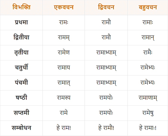
The figure illustrates different forms of the word "Rama" in Sanskrit. Traditional models like Word2Vec treat each word as a distinct entity and represent them separately in vector space. However, this does not capture the fact that such words often originate from the same root. FastText (P. Bojanowski et al.), an extension of the Skip-gram model proposed by (T. Mikolov et al.), addresses this limitation by incorporating subword information using character n-grams.
FastText introduces two main innovations:
-
Subword representation:
Words are represented as a bag of character n-grams. For example, the word "
where" withn = 3is represented as:<wh, whe, her, ere, re>, where < and > are special boundary symbols. The complete word itself (e.g.,<where>) is also included in the set. -
Scoring function:
The scoring function for a word-context pair uses the sum of the word’s subword vector representations:
\( s(w, c) = \sum_{g \in G_w} \mathbf{z}_g^\top \mathbf{v}_c \)
where \( G_w \) is the set of n-grams for word \( w \), \( \mathbf{z}_g \) is the vector for n-gram \( g \), and \( \mathbf{v}_c \) is the context word vector.
In practice, \( n \) is chosen such that \( 3 \leq n \leq 6 \).
The objective function of the original continuous Skip-gram model is to maximize the log-likelihood of context words given a center word:
\( \sum_{t=1}^{T} \sum_{c \in C_t} \log p(w_c \mid w_t) \)
FastText optimizes this objective using negative sampling (also from Mikolov et al.), reframing the task as a set of independent binary classification problems:
\( \sum_{t=1}^{T} \sum_{c \in C_t} \left[ \ell(s(w_t, w_c)) + \sum_{n \in N_{t,c}} \ell(-s(w_t, n)) \right] \)
Here:
- \( C_t \): the context window around the center word \( w_t \)
- \( N_{t,c} \): a set of negatively sampled words from the vocabulary
- \( \ell(x) = \log(1 + e^{-x}) \): the logistic loss function
This approach allows FastText to better represent rare and morphologically complex words by sharing representations across similar subword units.
References
- T. Mikolov et al., “Efficient estimation of word representations in vector space,” arXiv preprint arXiv:1301.3781, Jan. 2013.
- P. Bojanowski et al., “Enriching word vectors with subword information,” Transactions of the Association for Computational Linguistics, vol. 5, pp. 135–146, 2017.
- J. Pennington et al., “GloVe: Global vectors for word representation,” in Proc. Conf. Empirical Methods in Natural Language Processing (EMNLP), Doha, Qatar, 2014, pp. 1532–1543.
- CodeEmporium, “Word2Vec, GloVe, FastText – EXPLAINED!,” YouTube, Feb. 10, 2021. [Online]. Available: https://www.youtube.com/watch?v=ERibwqs9p38
- Krish Naik, Live NLP Playlist, YouTube playlist, 18 videos, 2022. [Online]. Available: https://www.youtube.com/playlist?list=PLZoTAELRMXVNNrHSKv36Lr3_156yCo6Nn