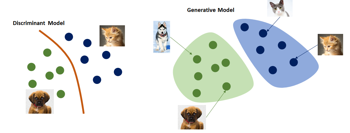
Generative Models

Generative models aim to learn the underlying distribution of each class unlike the discriminative models. The objective is to estimate the probability of generating an image from the joint distribution \( p(x, y) \), particularly when \( y = 1 \) or \( y = -1 \).

Implicit vs Explicit Generative Models

• Implicit Generative Models
  • Give up estimating the explicit form of \( p(x) \)
  • Aim only to sample images from the model; no explicit likelihood assignment
  • Capable of generating high-quality samples
  • Support fast sampling speeds
• Explicit Generative Models
  • Write an explicit function \( p(x) = f(x, \theta) \)
  • Input: Image \( x \)
  • Output: Likelihood value for image
  • Parameter: Weights \( \theta \)
  • Assign explicit likelihoods to images
  • Enables tasks like outlier detection
  • Often compromises image quality or sampling speed

Explicit models struggle with low fidelity in generated images and often underperform compared to implicit models.

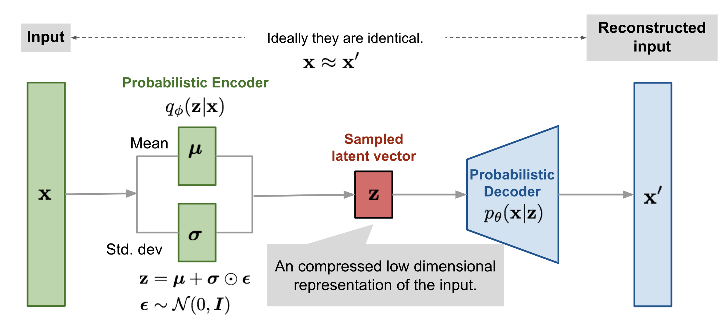
Variational Autoencoder (VAE)

A Variational Autoencoder is a type of generative model that learns a latent representation of data and can be used to generate similar data samples. While VAEs were originally used for images, changing the decoder enables them to generate text or other data types.

Main Motivation

Given a training dataset of faces, a neural network can be trained to model the distribution of the latent (hidden) semantic features that describe those faces. Once trained, we can sample new latent features and decode them to generate similar, realistic faces.

For the dataset \( X \), the goal is to maximize the likelihood of the data under the model: \( p(X) \). By marginalizing over latent variables \( z \), we write:

For a single data point:

Computing this integral exactly is intractable. Thus, we use sampling-based techniques that focus on the regions of \( z \) that significantly contribute to the probability mass of \( p(x, z) \).

Sampling Techniques

1. Monte Carlo Sampling

Most values of \( z \) contribute negligibly to \( p(x, z) \), so instead of averaging over all possible \( z \), we approximate the integral using samples:

2. Importance Sampling

Rather than sampling \( z \) uniformly, we sample from a distribution \( q(z) \) that is closer to the posterior. This improves the efficiency of the estimate:

Likelihood Estimator & ELBO Derivation

The marginal likelihood of a single data point \( x \) (parameterized by \( \theta \)) is:

For i.i.d. data \( X = \{x^{(1)}, \dots, x^{(m)}\} \), the total data likelihood is:

Step-by-Step Derivation Using Jensen's Inequality

1. Rewrite the log-likelihood using importance sampling:
   \[ \log p(x; \theta) = \log \left( \int q_\phi(z|x) \cdot \frac{p(x, z)}{q_\phi(z|x)} dz \right) = \log \mathbb{E}_{z \sim q_\phi(z|x)} \left[ \frac{p(x, z)}{q_\phi(z|x)} \right] \]
2. Apply Jensen’s inequality (since log is concave):
   \[ \log \mathbb{E}_{z \sim q_\phi(z|x)} \left[ \frac{p(x, z)}{q_\phi(z|x)} \right] \geq \mathbb{E}_{z \sim q_\phi(z|x)} \left[ \log \left( \frac{p(x, z)}{q_\phi(z|x)} \right) \right] \]
3. Decompose the right-hand side (ELBO):
   \[ \mathcal{L}(x; \theta, \phi) = \mathbb{E}_{z \sim q_\phi(z|x)} \left[ \log p_\theta(x|z) \right] - D_{KL}(q_\phi(z|x) \| p(z)) \]
4. Condition for equality:
   \[ \log p(x) = \mathbb{E}_{z \sim p(z|x)} \left[ \log \left( \frac{p(x, z)}{p(z|x)} \right) \right] = \log p(x) \]

   The inequality becomes equality when \( q_\phi(z|x) = p(z|x) \), i.e., the approximate posterior equals the true posterior.

Approximate Posterior via Neural Network

To approximate \( p(z|x) \), we define \( q_\phi(z|x) \) as a neural network that outputs a Gaussian distribution with mean and variance conditioned on \( x \):

We typically assume a standard normal prior:

The encoder (inference network) learns \( q_\phi(z|x) \), while the decoder models \( p_\theta(x|z) \).

Generation Process

Once trained, we can generate new samples as follows:

1. Sample \( z \sim p(z) = \mathcal{N}(0, I) \)
2. Generate \( x \sim p_\theta(x|z) \) using the decoder

The joint distribution used during training is:

Final / Overall Loss Function (ELBO):

KL Divergence Loss:

Given:

KL divergence:

Using log-density of multivariate Gaussians:

For \( q_\phi(z|x) = \mathcal{N}(\mu_\phi(x), \sigma_\phi^2(x)I) \), the closed-form KL divergence:

Rewriting to match the ELBO loss expression (with negative sign):

Reconstruction Loss Gradient Derivation:

Reparameterization Trick:

The VAE is a high-variance model due to stochastic sampling, making it non-differentiable. To backpropagate through stochastic nodes, we use the reparameterization trick:

For Image Datasets:

• The encoder is typically a stack of convolutional layers that maps the input image to latent variables (mean and variance).
• The decoder consists of transposed convolutions (deconvolution layers) to reconstruct the image from the latent representation.
• Each sample from the latent space (determined by predicted \(\mu_\phi(x)\) and \(\sigma_\phi(x)\)) results in a potentially different reconstructed image.